Code
suppressPackageStartupMessages(library(tidyverse))These visualizations are intended as a way to test the integrity and utility of the data export and cleaning workflow.
suppressPackageStartupMessages(library(tidyverse))screen_df <- readr::read_csv(file.path(here::here(), "data/csv/screening/agg/PLAY-screening-datab-latest.csv"))Rows: 933 Columns: 68
── Column specification ────────────────────────────────────────────────────────
Delimiter: ","
chr (55): session_name, session_release, participant_ID, participant_gender...
dbl (9): session_id, vol_id, child_age_mos, child_birthage, child_weight_p...
lgl (1): pilot_pilot
dttm (1): submit_date
date (2): session_date, participant_birthdate
ℹ Use `spec()` to retrieve the full column specification for this data.
ℹ Specify the column types or set `show_col_types = FALSE` to quiet this message.To calculate cumulative screening/recruiting calls by site, we have to add an index variable
df <- screen_df |>
  dplyr::arrange(submit_date) %>%
dplyr::mutate(n_calls = seq_along(submit_date))df |>
dplyr::filter(!is.na(submit_date), !is.na(n_calls), !is.na(site_id)) %>%
ggplot() +
aes(submit_date, n_calls, color = site_id) +
geom_point()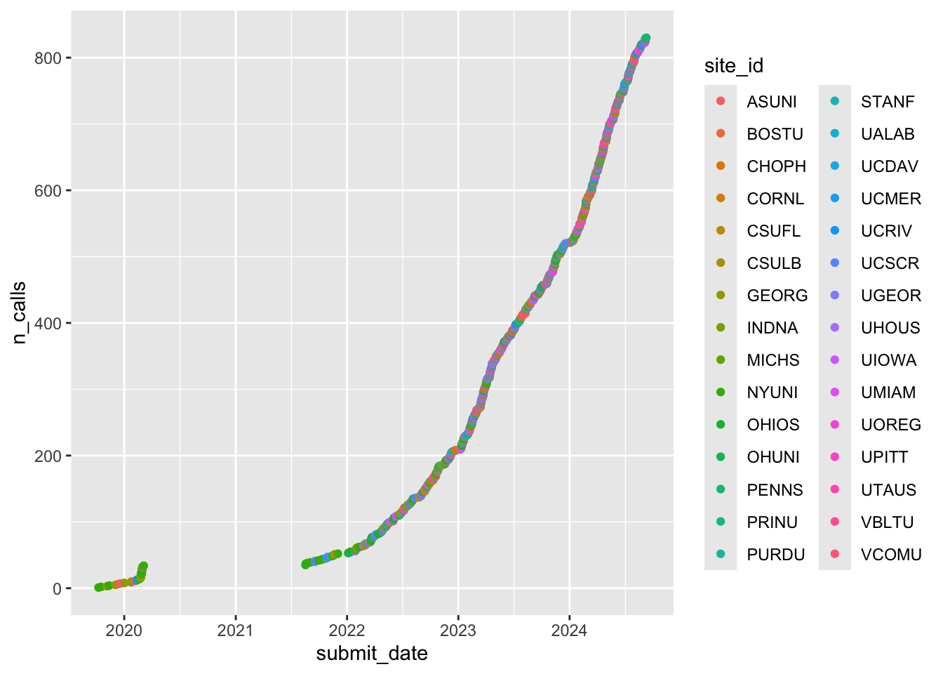
calls_by_site_plot <- function(df) {
  df |>
    filter(!is.na(site_id)) %>%
    ggplot() +
    aes(fct_infreq(site_id), fill = site_id) +
    geom_bar() +
    theme(axis.text.x = element_text(
      angle = 90,
      vjust = 0.5,
      hjust = 1
    )) + # Rotate text
    labs(x = "site") +
    theme(legend.position = "none")
}

calls_by_site_plot(df)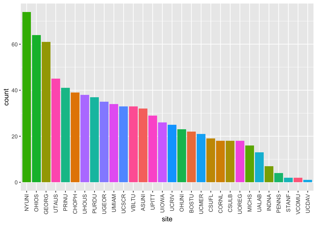
Child age in months (child_age_mos) by child_sex.
screen_df |>
  dplyr::filter(!is.na(child_age_mos), !is.na(child_sex)) |>
  ggplot() +
  aes(child_age_mos, fill = child_sex) +
  geom_histogram(bins = 50) +
  facet_grid(cols = vars(child_sex)) +
  theme(legend.position = "none")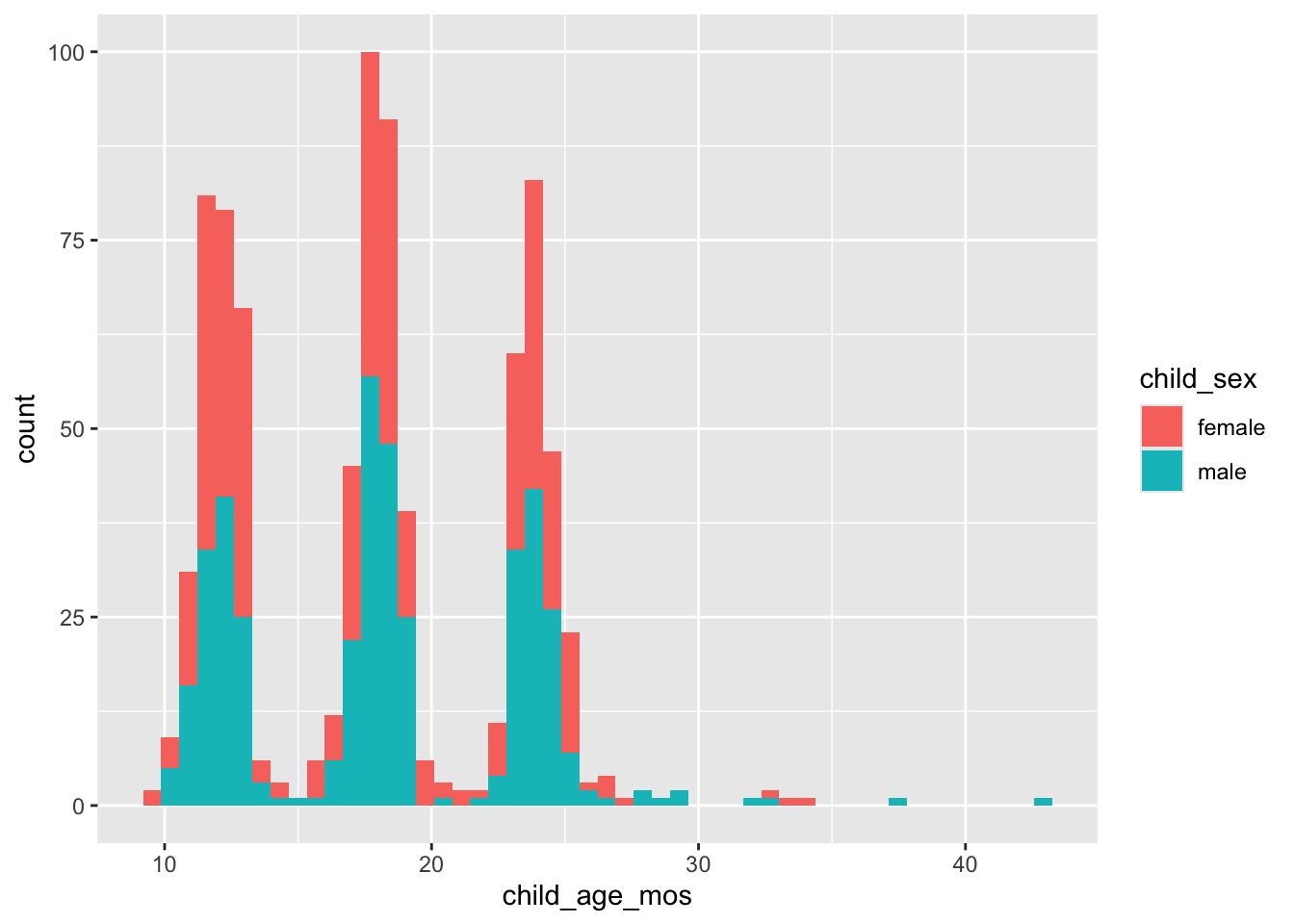
Some of the code to clean the screen_df variables could be incorporated into an earlier stage of the workflow.
Language(s) spoken to child by child_sex.
df <- screen_df |>
  dplyr::mutate(
    language_spoken_child = stringr::str_replace_all(language_spoken_child, " ", "_"),
    language_spoken_home = stringr::str_replace_all(language_spoken_home, " ", "_")
  )

xtabs(formula = ~ child_sex + language_spoken_child,
      data = df)
language_spoken_child
child_sex english english_other english_spanish english_spanish_other spanish
female 332 3 59 3 20
male 324 6 66 1 15xtabs(formula = ~ language_spoken_home + child_sex, data = df) child_sex
language_spoken_home female male
english 339 306
english_other 5 4
english_spanish 50 81
english_spanish_other 1 2
other 1 3
spanish 17 15xtabs(formula = ~ language_spoken_child + language_spoken_home, data = df) language_spoken_home
language_spoken_child english english_other english_spanish
english 618 3 25
english_other 3 6 0
english_spanish 19 0 94
english_spanish_other 3 0 1
spanish 2 0 11
language_spoken_home
language_spoken_child english_spanish_other other spanish
english 2 2 5
english_other 0 0 0
english_spanish 1 2 5
english_spanish_other 0 0 0
spanish 0 0 22xtabs(formula = ~ child_sex + child_bornonduedate,
data = screen_df) child_bornonduedate
child_sex no yes
female 8 404
male 9 402There are n=110 NAs.
screen_df |>
  dplyr::filter(is.na(child_bornonduedate)) |>
  dplyr::select(vol_id, participant_ID) |>
knitr::kable(format = 'html')| vol_id | participant_ID |
|---|---|
| 1656 | 001 |
| 1656 | 042 |
| 1656 | 043 |
| 1656 | 045 |
| 1656 | 046 |
| 1656 | 047 |
| 1008 | 013 |
| 1008 | 013 |
| 1008 | 013 |
| 1008 | 013 |
| 1008 | 020 |
| 1576 | 003 |
| 1576 | 006 |
| 1576 | 027 |
| 1576 | 028 |
| 1576 | 029 |
| 1576 | 030 |
| 1481 | 006 |
| 954 | 001 |
| 954 | 076 |
| 954 | 077 |
| 954 | 078 |
| 954 | 079 |
| 954 | 080 |
| 954 | 081 |
| 954 | 082 |
| 1590 | 015 |
| 1590 | 016 |
| 1590 | 017 |
| 899 | 088 |
| 899 | 089 |
| 899 | 090 |
| 899 | 091 |
| 899 | 092 |
| 899 | 094 |
| 1103 | 001 |
| 1596 | 013 |
| 1596 | 024 |
| 1596 | 025 |
| 1596 | 026 |
| 1596 | 027 |
| 1596 | 028 |
| 1596 | 030 |
| 1596 | 031 |
| 1596 | 032 |
| 1596 | 033 |
| 1596 | 034 |
| 1596 | 035 |
| 1657 | 003 |
| 1657 | 007 |
| 1657 | 008 |
| 1657 | 009 |
| 1657 | 010 |
| 979 | 026 |
| 1696 | 016 |
| 1696 | 017 |
| 1696 | 018 |
| 1696 | 019 |
| 1696 | 020 |
| 1705 | 023 |
| 1705 | 024 |
| 1705 | 025 |
| 1705 | 027 |
| 1705 | 026 |
| 1705 | 028 |
| 1705 | 029 |
| 1705 | 030 |
| 966 | 026 |
| 966 | 027 |
| 966 | 028 |
| 966 | 029 |
| 966 | 030 |
| 1422 | 031 |
| 1422 | 032 |
| 1422 | 033 |
| 1422 | 034 |
| 996 | 015 |
| 1459 | 019 |
| 1459 | 020 |
| 1459 | 021 |
| 1459 | 022 |
| 1459 | 023 |
| 1459 | 024 |
| 1459 | 025 |
| 1459 | 026 |
| 1459 | 027 |
| 1459 | 028 |
| 1459 | 029 |
| 1459 | 030 |
| 1459 | 031 |
| 1459 | 032 |
| 1459 | 033 |
| 1459 | 034 |
| 1663 | 033 |
| 1663 | 034 |
| 1663 | 035 |
| 1663 | 036 |
| 1663 | 037 |
| 1663 | 038 |
| 1663 | 040 |
| 1663 | 041 |
| 1517 | 056 |
| 1517 | 057 |
| 1517 | 058 |
| 1517 | 059 |
| 1517 | 060 |
| 1517 | 061 |
| 1517 | 062 |
| 1517 | 063 |
| 1517 | 064 |
xtabs(formula = ~ child_bornonduedate + child_onterm,
data = screen_df) child_onterm
child_bornonduedate no yes
no 1 16
yes 1 697Must convert pounds and ounces to decimal pounds.
df <- screen_df %>%
  dplyr::mutate(.,
                birth_weight_lbs = child_weight_pounds + child_weight_ounces/16)

df |>
  dplyr::filter(!is.na(birth_weight_lbs), !is.na(child_sex)) |>
  dplyr::filter(birth_weight_lbs > 0) |>
  ggplot() +
  aes(x = birth_weight_lbs, fill = child_sex) +
  geom_histogram(binwidth = 0.33) +
  facet_grid(cols = vars(child_sex)) +
  theme(legend.position = "none")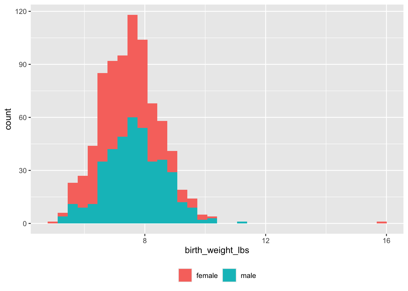
xtabs(formula = ~ child_sex + child_birth_complications,
      data = screen_df)
child_birth_complications
child_sex no yes
female 374 38
male 379 28There are some first names in the child_birth_complications_specify field, so it is not shown here.
screen_df |>
  dplyr::filter(!is.na(child_birth_complications_specify)) |>
  dplyr::select(child_age_mos, child_sex, child_birth_complications_specify) |>
  dplyr::arrange(child_age_mos) |>
knitr::kable(format = 'html')xtabs(formula = ~ child_sex + child_major_illnesses_injuries,
data = screen_df) child_major_illnesses_injuries
child_sex no yes
female 398 14
male 393 14screen_df |>
dplyr::filter(!is.na(child_illnesses_injuries_specify),
!stringr::str_detect(child_illnesses_injuries_specify, "OK")) |>
dplyr::select(child_age_mos, child_sex, child_illnesses_injuries_specify) |>
dplyr::arrange(child_age_mos) |>
knitr::kable(format = 'html')| child_age_mos | child_sex | child_illnesses_injuries_specify |
|---|---|---|
| 11.40697 | female | COVID in January, no later complications. |
| 11.86719 | female | RSV when she 3 months; was in hospital for 2 nights |
| 12.68902 | female | fractured wrist when she was 9 months |
| 12.72189 | female | At 2 months got RSV viral infection and was in hospital for 4 days. At 5 months feel off the bed and hit her head. Ended up in the emergency room but exams showed she was okay. Neither of these events resulted in any motor, perceptual, or cognitive impairment or delay as a result. |
| 12.73285 | male | He had Covid once. |
| 12.76162 | female | RSV when 10 weeks old, hospitalized for 1 week |
| 13.01775 | male | Covid in December but this did NOT result in a visual, auditory, motor, or cognitive disability according to mom |
| 13.02186 | male | Respiratory failure and sepsis after birth that was resolved |
| 16.17494 | female | Child had a fall but she was fine. |
| 17.81860 | female | **bit by tick a couple months ago, took meds to prevent Lyme disease |
| 17.88160 | male | Covid in November |
| 18.04597 | female | broke leg in April - all healed now. slide accident, she was 16 months. in a cast for three weeks, and then a week phantom limping. |
| 18.18020 | female | Respiratory Syncytial Virus(RSV) |
| 18.67330 | male | tibial stress factor |
| 18.70617 | male | RSV but did not need to be admitted. This illness did not result in an impairment or disability. |
| 18.77055 | male | Child had COVID twice (fever, etc.) |
| 20.67856 | male | Anaphylactic reaction to peanuts |
| 22.48658 | female | Child was born with a heart murmur- cardiologist said she is unaffected and will likely grow out of it. Child also had an isolated febrile seizure short after 1st birthday. Has not experienced a seizure since. |
| 23.01118 | male | He had RSV then COVID around 13-14 months old, but they were both very mild. No complications arose from either. |
| 23.20979 | female | febrile seizure- around 1 1/2 years |
| 23.33991 | male | split lip open in March after falling on hardwood -- preventative antibiotics, all clear |
| 24.03024 | male | had COVID at 7 months |
| 24.06312 | female | Pneumonia , was in the hospital for one night, this did not result in anything |
| 24.91782 | female | She had COVID, and when she was little had an cardiac issue (her heart was "working" too hard) but she was okay soon after (this was first 2-3 months after birth). March of 2021 she had fully recovered from this, and received treatment |
| 25.70814 | male | hospital day 4 for hypothermia - then negative / no diagnosis |
| 26.76008 | male | Has had a fall, was a concussion but not diagnosed with any disabilities |
| 32.67724 | male | Pneumonia at 5 months |
xtabs(formula = ~ child_sex + child_vision_disabilities,
      data = screen_df)
child_vision_disabilities
child_sex no yes
female 409 3
male 405 2screen_df |>
dplyr::filter(!is.na(child_vision_disabilities_specify)) |>
dplyr::select(child_age_mos, child_sex, child_vision_disabilities_specify) |>
dplyr::arrange(child_age_mos) |>
knitr::kable(format = 'html')| child_age_mos | child_sex | child_vision_disabilities_specify |
|---|---|---|
| 18.70617 | male | He wears glasses to correct his far sighted vision. He does not have vision loss. |
| 18.90204 | female | Duane's Syndrome in left eye |
| 22.35371 | female | She has a lazy eye, she wears an eye patch for part of the day. |
| 23.14267 | female | Strabismus - wears glasses |
| 24.03024 | male | lazy eye but corrected |
xtabs(formula = ~ child_sex + child_hearing_disabilities,
      data = screen_df)
child_hearing_disabilities
child_sex no yes
female 412 0
male 406 1screen_df |>
dplyr::filter(!is.na(child_hearing_disabilities_specify)) |>
dplyr::select(child_age_mos, child_sex, child_hearing_disabilities_specify) |>
dplyr::arrange(child_age_mos) |>
knitr::kable(format = 'html')| child_age_mos | child_sex | child_hearing_disabilities_specify |
|---|---|---|
| 32.67724 | male | Temporary hearing loss so tubes in his ears, one still remaining |
xtabs(formula = ~ child_sex + child_developmentaldelays,
      data = screen_df)
child_developmentaldelays
child_sex no yes
female 350 3
male 349 5There may be first names in the child_developmentaldelays_specify field, so it is not shown here.
screen_df |>
  dplyr::filter(!is.na(child_developmentaldelays_specify)) |>
  dplyr::select(child_age_mos, child_sex, child_developmentaldelays_specify) |>
  dplyr::arrange(child_age_mos) |>
knitr::kable(format = 'html')This is work yet-to-be-done. The time stamps need to be reformatted prior to visualization.
extract_sleep_hr <- function(t) {
  t |>
    stringr::str_extract("^[0-9]{2}\\:[0-9]{2}\\:[0-9]{2}") |>
    hms::as_hms()
}

df <- screen_df |>
  dplyr::mutate(child_sleep_time = extract_sleep_hr(child_sleep_time)) |>
  dplyr::filter(!is.na(child_sleep_time))

df |>
  dplyr::filter(!is.na(child_sleep_time),
                !is.na(child_sex),
                !is.na(child_sleep_location)) |>
  ggplot() +
  aes(child_sleep_time, fill = child_sex) +
  geom_histogram(bins = 18) +
  facet_grid(rows = vars(child_sex), cols = vars(child_sleep_location)) +
  theme(legend.position = "none") +
  theme(axis.text.x = element_text(angle = 90))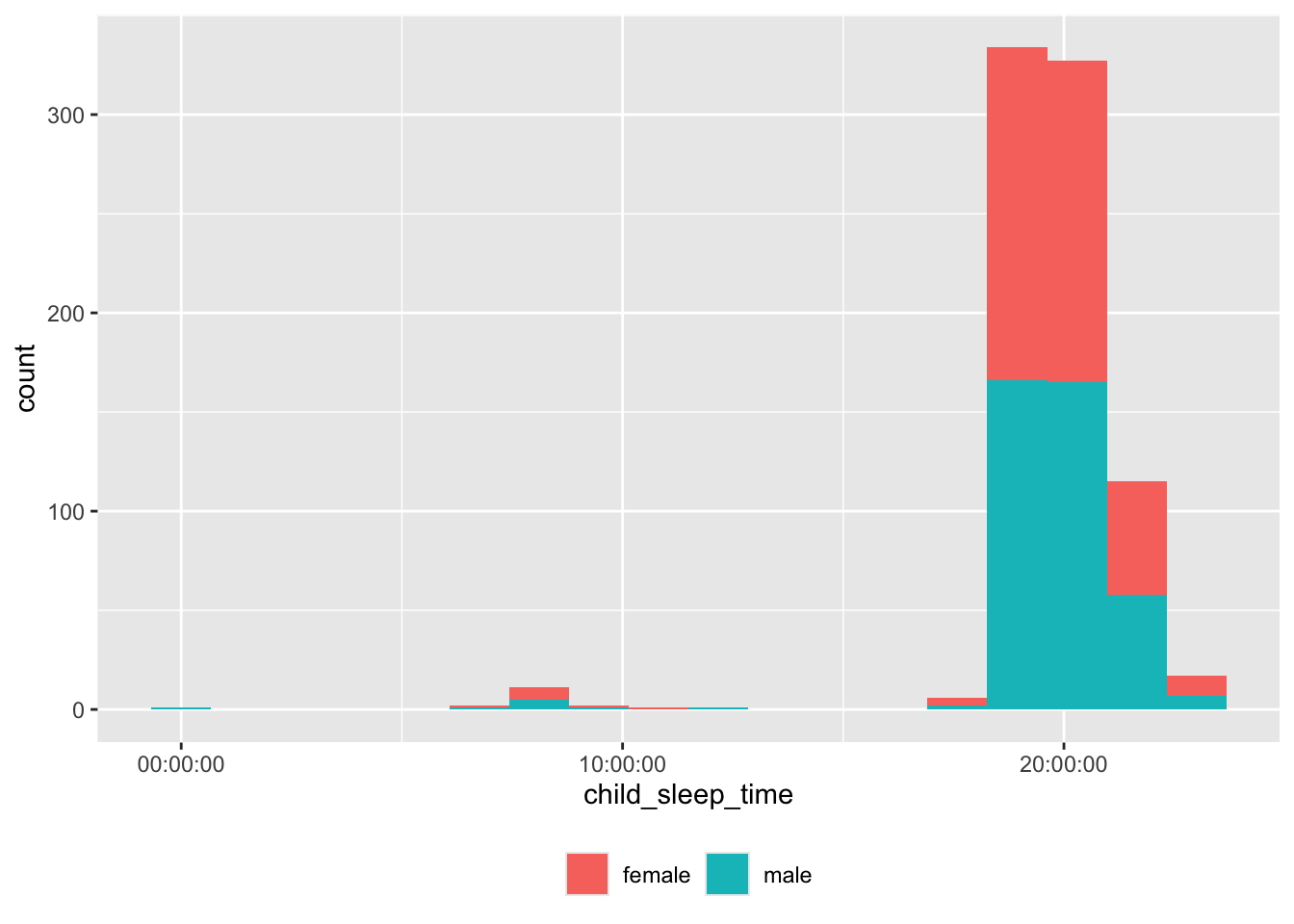
df |>
  dplyr::filter(!is.na(child_sleep_time),
                !is.na(child_sex),
                !is.na(child_sleep_location)) |>
  ggplot() +
  aes(child_sleep_time, child_age_mos, color = child_sex) +
  facet_grid(cols = vars(child_sex)) +
  geom_point(alpha = .3) +
  theme(legend.position = "none") +
  theme(axis.text.x = element_text(angle = 90))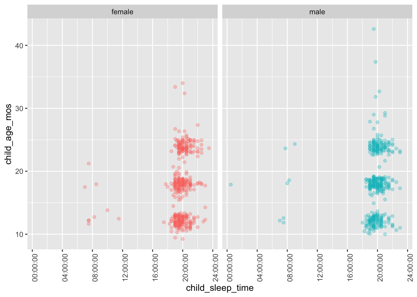
Some of the bed times are probably not in correct 24 hr time.
df |>
  dplyr::filter(child_sleep_time < hms::as_hms("16:00:00")) |>
  dplyr::select(site_id, participant_ID, child_sleep_time) |>
  dplyr::arrange(site_id, participant_ID) |>
knitr::kable('html')| site_id | participant_ID | child_sleep_time |
|---|---|---|
| CSUFL | 013 | 07:00:00 |
| CSULB | 006 | 07:30:00 |
| INDNA | 004 | 09:00:00 |
| INDNA | 006 | 07:45:00 |
| NYUNI | 082 | 07:00:00 |
| OHIOS | 002 | 10:00:00 |
| OHUNI | 020 | 07:30:00 |
| PRINU | 001 | 12:15:00 |
| PRINU | 018 | 07:30:00 |
| PRINU | 027 | 07:30:00 |
| PRINU | 043 | 08:15:00 |
| PURDU | 020 | 08:30:00 |
| PURDU | 021 | 11:30:00 |
| UCSCR | 011 | 07:30:00 |
| UGEOR | 016 | 07:30:00 |
| UPITT | 013 | 08:15:00 |
| UPITT | 016 | 00:30:00 |
| UTAUS | 023 | 08:00:00 |
df <- screen_df |>
  dplyr::mutate(child_wake_time = extract_sleep_hr(child_wake_time)) |>
  dplyr::filter(!is.na(child_wake_time))

df |>
  dplyr::filter(!is.na(child_wake_time),
                !is.na(child_sex),
                !is.na(child_sleep_location)) |>
  ggplot() +
  aes(child_wake_time, fill = child_sex) +
  geom_histogram(bins = 18) +
  facet_grid(rows = vars(child_sex), cols = vars(child_sleep_location)) +
  theme(legend.position = "none") +
  theme(axis.text.x = element_text(angle = 90))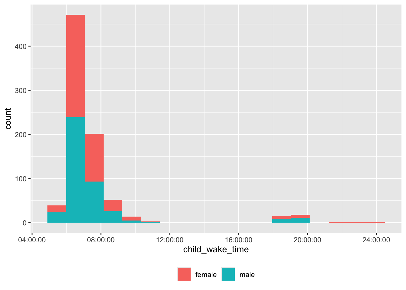
There are some unusual wake times, too.
df |>
  dplyr::filter(child_wake_time > hms::as_hms("16:00:00")) |>
  dplyr::select(site_id, participant_ID, child_wake_time) |>
  dplyr::arrange(site_id, participant_ID) |>
knitr::kable('html')| site_id | participant_ID | child_wake_time |
|---|---|---|
| BOSTU | 001 | 19:30:00 |
| CHOPH | 017 | 19:30:00 |
| CORNL | 016 | 19:50:00 |
| GEORG | 026 | 19:00:00 |
| OHIOS | 009 | 18:30:00 |
| OHIOS | 012 | 19:30:00 |
| OHIOS | 014 | 18:30:00 |
| OHIOS | 018 | 18:45:00 |
| OHIOS | 019 | 19:30:00 |
| OHIOS | 021 | 19:30:00 |
| OHIOS | 029 | 19:30:00 |
| OHIOS | 031 | 19:30:00 |
| OHIOS | 035 | 19:00:00 |
| OHIOS | 062 | 18:30:00 |
| PRINU | 015 | 19:00:00 |
| PRINU | 018 | 19:45:00 |
| PRINU | 027 | 20:00:00 |
| PRINU | 043 | 19:00:00 |
| PURDU | 020 | 21:30:00 |
| PURDU | 021 | 23:30:00 |
| PURDU | 023 | 23:00:00 |
| UALAB | 009 | 18:00:00 |
| UALAB | 013 | 20:00:00 |
| UCRIV | 007 | 18:00:00 |
| UCSCR | 035 | 18:30:00 |
| UGEOR | 002 | 19:30:00 |
| UHOUS | 014 | 19:00:00 |
| UMIAM | 013 | 20:00:00 |
| UMIAM | 029 | 19:30:00 |
| UMIAM | 041 | 20:00:00 |
| UPITT | 018 | 19:15:00 |
| UTAUS | 013 | 18:00:00 |
| UTAUS | 020 | 18:30:00 |
| UTAUS | 040 | 19:00:00 |
| UTAUS | 043 | 19:15:00 |
| VBLTU | 025 | 19:15:00 |
df <- screen_df |>
  dplyr::mutate(child_sleep_time = extract_sleep_hr(child_sleep_time),
                  child_wake_time = extract_sleep_hr(child_wake_time)) |>
  dplyr::filter(!is.na(child_sleep_time),
                !is.na(child_wake_time)) |>
  dplyr::mutate(child_sleep_secs = (child_sleep_time - child_wake_time))

df |>
  dplyr::filter(!is.na(child_sleep_secs),
                !is.na(child_sleep_location)) |>
  dplyr::mutate(sleep_hrs = child_sleep_secs/(60*60)) |>
  ggplot() +
  aes(sleep_hrs, fill = child_sex) +
  geom_histogram(bins = 18) +
  facet_grid(rows = vars(child_sex), cols = vars(child_sleep_location)) +
  theme(legend.position = "none") +
  theme(axis.text.x = element_text(angle = 90))
Don't know how to automatically pick scale for object of type <difftime>.
Defaulting to continuous.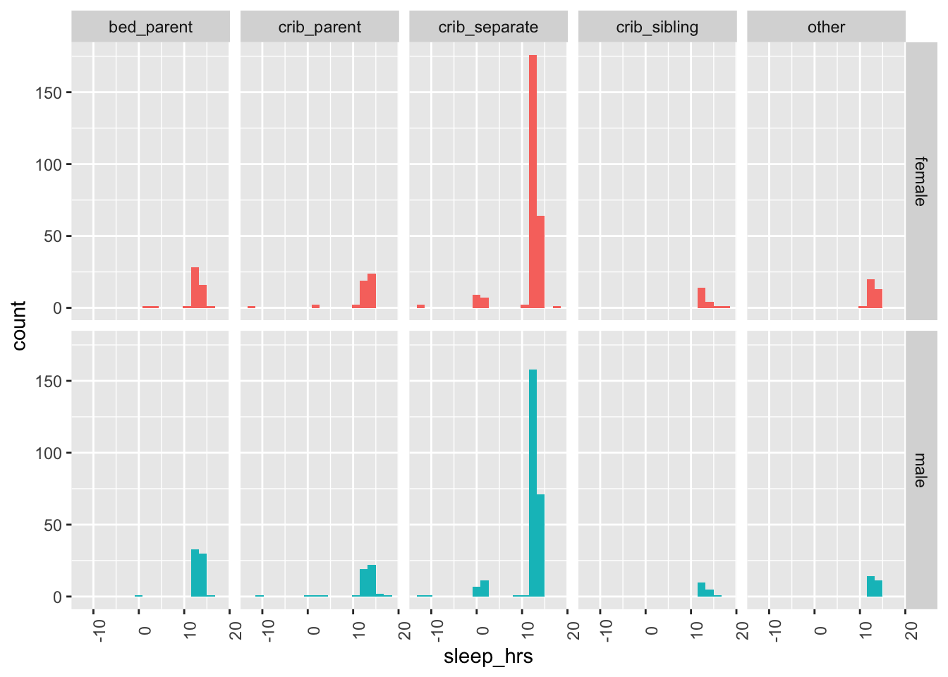
df |>
  dplyr::filter(!is.na(child_sleep_secs),
                !is.na(child_sleep_location)) |>
  dplyr::mutate(sleep_hrs = child_sleep_secs/(60*60)) |>
  ggplot() +
  aes(child_age_mos, sleep_hrs, color = child_sex) +
  geom_point(alpha = .2) +
  facet_grid(rows = vars(child_sex), cols = vars(child_sleep_location)) +
  theme(legend.position = "none") +
  theme(axis.text.x = element_text(angle = 90))
Don't know how to automatically pick scale for object of type <difftime>.
Defaulting to continuous.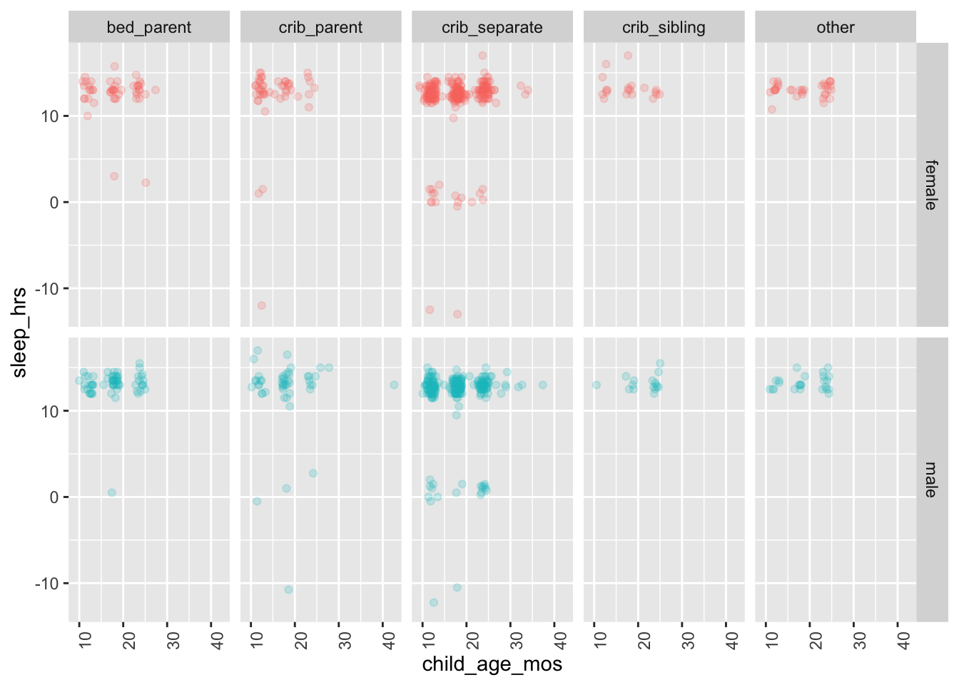
Again, there are some unusual values.
df |>
  dplyr::filter(child_sleep_secs < 12000) |>
  dplyr::select(site_id, participant_ID, child_sleep_time, child_wake_time, child_sleep_secs) |>
  dplyr::arrange(site_id, participant_ID) |>
knitr::kable('html')| site_id | participant_ID | child_sleep_time | child_wake_time | child_sleep_secs |
|---|---|---|---|---|
| BOSTU | 001 | 19:30:00 | 19:30:00 | 0 secs |
| CHOPH | 017 | 20:45:00 | 19:30:00 | 4500 secs |
| CORNL | 016 | 20:05:00 | 19:50:00 | 900 secs |
| CSUFL | 013 | 07:00:00 | 06:00:00 | 3600 secs |
| CSULB | 006 | 07:30:00 | 07:30:00 | 0 secs |
| GEORG | 026 | 19:45:00 | 19:00:00 | 2700 secs |
| INDNA | 004 | 09:00:00 | 08:00:00 | 3600 secs |
| INDNA | 006 | 07:45:00 | 06:30:00 | 4500 secs |
| NYUNI | 082 | 07:00:00 | 06:15:00 | 2700 secs |
| OHIOS | 002 | 10:00:00 | 08:00:00 | 7200 secs |
| OHIOS | 009 | 18:30:00 | 18:30:00 | 0 secs |
| OHIOS | 012 | 20:00:00 | 19:30:00 | 1800 secs |
| OHIOS | 014 | 20:00:00 | 18:30:00 | 5400 secs |
| OHIOS | 018 | 20:00:00 | 18:45:00 | 4500 secs |
| OHIOS | 019 | 20:30:00 | 19:30:00 | 3600 secs |
| OHIOS | 021 | 20:00:00 | 19:30:00 | 1800 secs |
| OHIOS | 029 | 20:45:00 | 19:30:00 | 4500 secs |
| OHIOS | 031 | 20:30:00 | 19:30:00 | 3600 secs |
| OHIOS | 035 | 20:30:00 | 19:00:00 | 5400 secs |
| OHIOS | 062 | 20:30:00 | 18:30:00 | 7200 secs |
| OHUNI | 020 | 07:30:00 | 06:00:00 | 5400 secs |
| PRINU | 015 | 19:00:00 | 19:00:00 | 0 secs |
| PRINU | 018 | 07:30:00 | 19:45:00 | -44100 secs |
| PRINU | 027 | 07:30:00 | 20:00:00 | -45000 secs |
| PRINU | 043 | 08:15:00 | 19:00:00 | -38700 secs |
| PURDU | 020 | 08:30:00 | 21:30:00 | -46800 secs |
| PURDU | 021 | 11:30:00 | 23:30:00 | -43200 secs |
| PURDU | 023 | 22:30:00 | 23:00:00 | -1800 secs |
| UALAB | 009 | 19:30:00 | 18:00:00 | 5400 secs |
| UALAB | 013 | 19:30:00 | 20:00:00 | -1800 secs |
| UCRIV | 007 | 21:00:00 | 18:00:00 | 10800 secs |
| UCSCR | 011 | 07:30:00 | 06:30:00 | 3600 secs |
| UCSCR | 035 | 20:45:00 | 18:30:00 | 8100 secs |
| UGEOR | 002 | 20:00:00 | 19:30:00 | 1800 secs |
| UGEOR | 016 | 07:30:00 | 08:00:00 | -1800 secs |
| UHOUS | 014 | 19:00:00 | 19:00:00 | 0 secs |
| UMIAM | 013 | 21:00:00 | 20:00:00 | 3600 secs |
| UMIAM | 029 | 20:00:00 | 19:30:00 | 1800 secs |
| UMIAM | 041 | 21:30:00 | 20:00:00 | 5400 secs |
| UPITT | 013 | 08:15:00 | 07:15:00 | 3600 secs |
| UPITT | 016 | 00:30:00 | 11:00:00 | -37800 secs |
| UPITT | 018 | 19:15:00 | 19:15:00 | 0 secs |
| UTAUS | 013 | 19:30:00 | 18:00:00 | 5400 secs |
| UTAUS | 020 | 20:00:00 | 18:30:00 | 5400 secs |
| UTAUS | 023 | 08:00:00 | 07:00:00 | 3600 secs |
| UTAUS | 040 | 19:00:00 | 19:00:00 | 0 secs |
| UTAUS | 043 | 22:00:00 | 19:15:00 | 9900 secs |
| VBLTU | 025 | 19:30:00 | 19:15:00 | 900 secs |
df <- screen_df |>
  dplyr::mutate(child_nap_hours = as.numeric(child_nap_hours)) |>
  dplyr::filter(!is.na(child_sleep_time))
Warning: There was 1 warning in `dplyr::mutate()`.
ℹ In argument: `child_nap_hours = as.numeric(child_nap_hours)`.
Caused by warning:
! NAs introduced by coerciondf |>
dplyr::filter(!is.na(child_nap_hours),
!is.na(child_sex)) |>
ggplot() +
aes(child_nap_hours, fill = child_sex) +
geom_histogram(bins = 18) +
facet_grid(cols = vars(child_sex)) +
theme(legend.position = "none")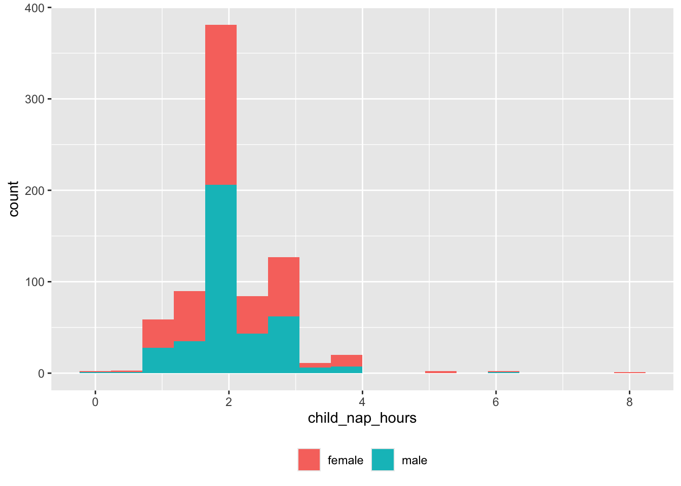
df |>
  dplyr::filter(!is.na(child_nap_hours),
                !is.na(child_sex)) |>
  ggplot() +
  aes(child_age_mos, child_nap_hours, color = child_sex) +
  geom_point(alpha = .3) +
  geom_smooth() +
  facet_grid(cols = vars(child_sex)) +
  theme(legend.position = "none")
`geom_smooth()` using method = 'loess' and formula = 'y ~ x'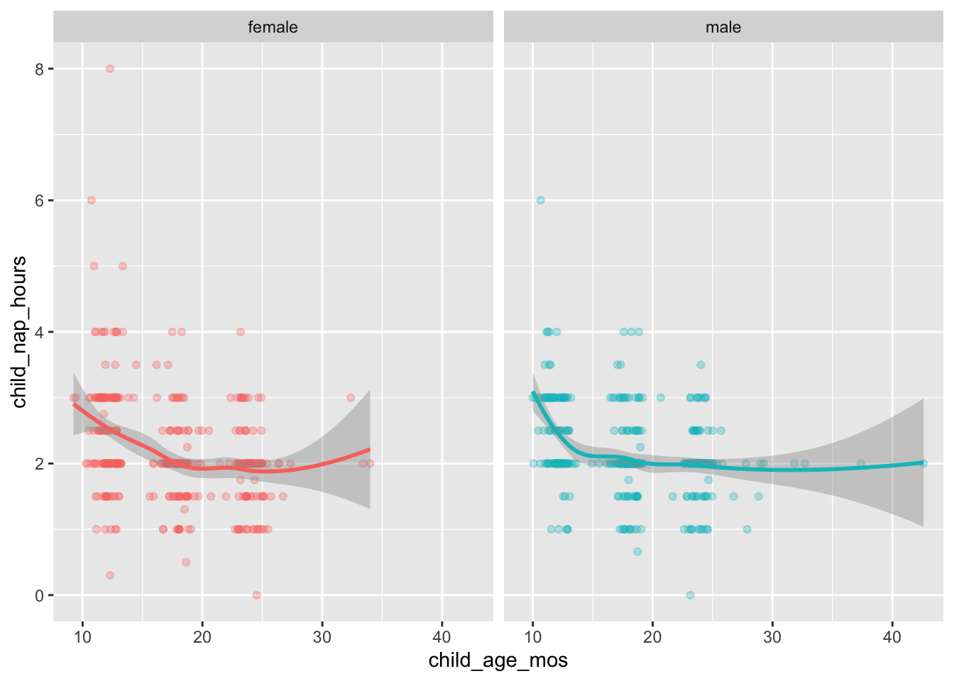
And there are some very long nappers or null values we need to capture.
df |>
  dplyr::filter(child_nap_hours > 5) |>
  dplyr::select(site_id, participant_ID, child_nap_hours) |>
  dplyr::arrange(site_id, participant_ID) |>
knitr::kable('html')| site_id | participant_ID | child_nap_hours |
|---|---|---|
| UMIAM | 003 | 8 |
| UOREG | 012 | 6 |
| UTAUS | 009 | 6 |
xtabs(formula = ~ child_sex + child_sleep_location,
data = screen_df)xtabs(formula = ~ child_sex + mom_bio,
data = screen_df) mom_bio
child_sex no_adoptive no_partnerchild yes
female 2 1 398
male 0 0 404screen_df |>
dplyr::filter(!is.na(mom_childbirth_age),
!is.na(child_sex)) |>
ggplot() +
aes(x = mom_childbirth_age, fill = child_sex) +
geom_histogram(bins = 25) +
facet_grid(cols = vars(child_sex)) +
theme(legend.position = "none")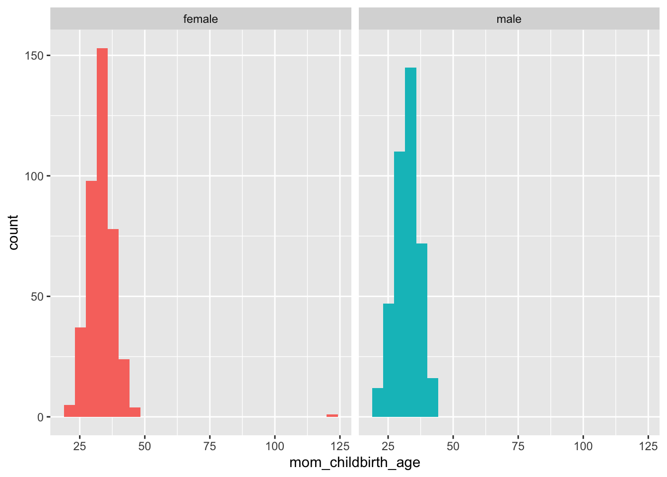
Clearly, there are some impossible (erroneous) maternal ages > 100. Here are details:
old_moms <- screen_df |>
  dplyr::filter(mom_childbirth_age > 55)

old_moms |>
  dplyr::select(submit_date, vol_id, participant_ID, mom_childbirth_age) |>
knitr::kable(format = 'html')| submit_date | vol_id | participant_ID | mom_childbirth_age |
|---|---|---|---|
| 2022-07-07 15:03:20 | 1391 | 005 | 121.22 |
df <- screen_df |>
  dplyr::filter(!is.na(mom_race)) |>
  dplyr::mutate(mom_race = dplyr::recode(
    mom_race,
    morethanone = "more_than_one",
    americanindian = "american_indian"))

xtabs(~mom_race, df)
mom_race
american_indian asian black more_than_one nativehawaiian
3 26 36 42 1
other refused white
50 2 652 df <- screen_df |>
dplyr::mutate(mom_birth_country = dplyr::recode(
mom_birth_country,
unitedstates = "US",
united_states = "US",
othercountry = "Other",
other_country = "Other",
refused = "Refused"
))
xtabs(~ mom_birth_country, data = df)mom_birth_country
Other puertorico US
89 3 720 df <- screen_df |>
dplyr::mutate(mom_birth_country_specify = stringr::str_to_title(mom_birth_country_specify)) |>
dplyr::filter(!is.na(mom_birth_country_specify)) |>
dplyr::select(child_sex, mom_birth_country_specify)
unique(df$mom_birth_country_specify) [1] "Mexico" "South Korea" "Argentina"
[4] "Spain" "Zimbabwe" "Canada"
[7] "Bolivia" "Uk" "Refused"
[10] "United Kingdom" "Liberia" "Pakistan"
[13] "Australia" "Venezuela" "India"
[16] "Kenya" "England" "China"
[19] "Ireland" "El Salvador" "Colombia"
[22] "Chile" "Haiti" "Guatemala"
[25] "Ecuador" "Guadalajara Mexico" "Costa Rica"
[28] "Italy" "Malaysia" "Phillipines"
[31] "Dominican Republic" "Nigeria" "Honduras"
[34] "Colomobia" "Columbia" "Peru"
[37] "Panama" df <- screen_df |>
dplyr::filter(!is.na(mom_education)) |>
dplyr::select(child_sex, mom_education)
xtabs(~ mom_education, data = df)mom_education
associates bachelor_s_deg bachelors diploma
28 1 263 28
doctorate eleventh ged graduate_nodegree
100 1 4 25
masters ninth professional somecollege
277 1 36 43
voc_diplima voc_nodiplima
3 1 This requires some recoding work.
df <- screen_df |>
  dplyr::filter(!is.na(mom_employment))

xtabs(~ mom_employment, data = df)
mom_employment
full_time no part_time
460 193 158 This information is available, but would need to be substantially recoded to be useful in summary form.
df <- screen_df |>
  dplyr::filter(!is.na(mom_jobs_number))

xtabs(~ mom_jobs_number, data = df)
mom_jobs_number
0 1 2 3 4 5more
1 552 61 1 1 1 df <- screen_df |>
dplyr::filter(!is.na(mom_jobs_number),
!is.na(mom_employment))
xtabs(~ mom_jobs_number + mom_employment, data = df) mom_employment
mom_jobs_number full_time part_time
0 0 1
1 420 132
2 37 24
3 1 0
4 1 0
5more 1 0df <- screen_df |>
dplyr::filter(!is.na(mom_training))
xtabs(~ mom_training, data = df)mom_training
no yes
789 20 df <- screen_df |>
dplyr::select(mom_childbirth_age, biodad_childbirth_age, biodad_race, child_sex) |>
dplyr::mutate(
biodad_race =
dplyr::recode(
biodad_race,
americanindian_NA = "american_indian",
asian_NA = "asian",
NA_asian = "asian",
black_NA = "black",
donotknow_NA = "do_not_know",
NA_NA = "NA",
NA_white = "white",
other_NA = "other",
refused_NA = "refused",
white_NA = "white",
morethanone_NA = "more_than_one"
)
) |>
dplyr::mutate(biodad_childbirth_age = stringr::str_remove_all(biodad_childbirth_age, "[_NA]")) |>
# dplyr::filter(!is.na(biodad_childbirth_age), !is.na(biodad_race)) |>
dplyr::mutate(biodad_childbirth_age = as.numeric(biodad_childbirth_age))Warning: There was 1 warning in `dplyr::mutate()`.
ℹ In argument: `biodad_childbirth_age = as.numeric(biodad_childbirth_age)`.
Caused by warning:
! NAs introduced by coercionxtabs(~ biodad_race, df)biodad_race
american_indian asian black do_not_know
4 29 43 5
more_than_one NA nativehawaiian_NA other
36 32 2 66
refused white
3 611 df |>
dplyr::filter(!is.na(biodad_childbirth_age),
!is.na(child_sex)) |>
ggplot() +
aes(x = biodad_childbirth_age, fill = child_sex) +
geom_histogram(bins = 25) +
facet_grid(cols = vars(child_sex)) +
theme(legend.position = "none")
df |>
  dplyr::filter(!is.na(biodad_childbirth_age),
                !is.na(mom_childbirth_age),
                !is.na(child_sex)) |>
  ggplot() +
  aes(x = mom_childbirth_age, y = biodad_childbirth_age, color = child_sex) +
  geom_point() +
  facet_grid(cols = vars(child_sex)) +
  theme(legend.position = "none")
df <- screen_df |>
  dplyr::filter(!is.na(childcare_types))

xtabs(~ childcare_types, data = df)
childcare_types
childcare nanny
231 1
nanny_home nanny_home childcare
42 13
nanny_home nanny_nothome nanny_home nanny_nothome relative
3 1
nanny_home relative nanny_nothome
7 15
nanny_nothome childcare nanny_nothome relative
3 3
none relative
191 95
relative childcare
19 This requires some cleaning.
df <- screen_df |>
  dplyr::filter(!is.na(childcare_hours)) |>
  dplyr::arrange(childcare_hours)

unique(df$childcare_hours)
[1] "1"
[2] "10"
[3] "12"
[4] "13"
[5] "14"
[6] "14.5"
[7] "15"
[8] "15-20"
[9] "16"
[10] "16-20"
[11] "17"
[12] "17.5"
[13] "18"
[14] "19"
[15] "2"
[16] "2-3"
[17] "2-4"
[18] "20"
[19] "20 hours"
[20] "20 hours a week - maternal grandmother"
[21] "21"
[22] "21 (14 hr childcare center, 7 hr babysitter)"
[23] "22"
[24] "24"
[25] "25"
[26] "25, 15 of those hours are at daycare"
[27] "26"
[28] "27"
[29] "28"
[30] "3"
[31] "30"
[32] "30-35"
[33] "30-40"
[34] "31"
[35] "32"
[36] "32-35"
[37] "33"
[38] "34"
[39] "35"
[40] "35-40"
[41] "36"
[42] "36; Grandpa watches one day a week"
[43] "37"
[44] "38"
[45] "4"
[46] "40"
[47] "40+"
[48] "40-45"
[49] "40-45 hours"
[50] "40-50"
[51] "42"
[52] "42.5"
[53] "43"
[54] "45"
[55] "45-50"
[56] "47"
[57] "5"
[58] "50"
[59] "52.5"
[60] "53"
[61] "6"
[62] "63"
[63] "7"
[64] "8"
[65] "8 hours with grandmother"
[66] "8-16"
[67] "8-5 each day"
[68] "8.5"
[69] "80"
[70] "9" This requires some cleaning.
df <- screen_df |>
  dplyr::filter(!is.na(childcare_language))

unique(df$childcare_language)
[1] "Spanish and English (half and half)"
[2] "English"
[3] "Spanish"
[4] "English and Spanish (50/50)"
[5] "english"
[6] "English when speaking with children, but Arabic when speaking to eachother"
[7] "Mostly English, some Spanish"
[8] "Mandarin"
[9] "Spanish at the center"
[10] "English (spanish around her)"
[11] "English and Spanish"
[12] "English, Spanish"
[13] "Usually English, sometimes arabic and french"
[14] "Bangladeshi"
[15] "English and speaks a little bit of Japanese but not directly to Lucas"
[16] "English and Creole"
[17] "Spanish (sometimes English)"
[18] "English;Spanish"
[19] "Spanish and English"
[20] "spanish"
[21] "French only"
[22] "English and some sign language"
[23] "Engish"
[24] "English, American Sign Language"
[25] "English and ASL"
[26] "Ingles"
[27] "English/Spanish"
[28] "English and some Spanish"
[29] "english, has been exposed to Arabic"
[30] "Nanny in Spanish at home. At school both English and Spanish."
[31] "English (majority of the time) and sometimes Spanish"
[32] "English and Spanish 50/50"
[33] "english, some spanish"
[34] "English, Italian, Spanish"
[35] "English, sometimes a little bit of Spanish"
[36] "English & Spanish"
[37] "English and Portuguese" This requires some cleaning.